Multinomial Logit Regression as PGM

I decided to switch to English as I believe that this topic may be interesting for a wider audience. In the last post I have given a simple example of how the t-test for independent samples can be understood from a generalized linear modeling (GLM) perspective, how the model translates into a probabilistic graphcal model (PGM) and how to use Bayesian estimation techniques for parameter estimation. The main motivation behind that post was to show, how generalized linear models, probabilistic graphical models and bayesian estimation techniques can work together for solving statistical inference tasks, particularly in but not limited to Psychology.

I can hear the one or the other say: “Pah, t-test, peanuts!”. So in this post I would like to turn to something a bit more advanced: Multinomial Logit Regression (MLR). One task of MLR is to model the probability of a categorical response $c$ out of a set of $C$ mutually exclusive possible responses based on a set of predictors that may characterize for example the repondents. Typical questions are: Which characteristics of a person predict the choice of a specific party (Political Science) or a specific product (Economics) or a specific category on a multiple choice questionaire (Psychology). This type of model is also quite prominent in the machine learning community. One task is to classify text documents into $C$ mutually exclusive categories based on a set of text features as predictors.

Before we can specify the model as a PGM, we should have a look at its formal structure. First we need a probability distribution that is capable of modeling the probabilty of a certain categorical response $c$ based on a set of parametetrs. One such distribution is:

(1) $\begin{equation*} p(y_i=c)=\frac{\mbox{exp}\left\{ \lambda_{ci}\right\}}{\sum_{c=1}^C\mbox{exp}\left\{ \lambda_{ci}\right\}}. \end{equation*}$

This is quite neat. The denominator of that distribution is sometimes called the partition function or in German Zustandssumme from its use in statistical physics. It ensures that the probabilites for the possible events, states or responses sum up to one. Please note that the distribiution above has a little identification problem that can be solved by either setting $\lambda_{1i}$ to zero or by imposing a sum constraint over the parameters.

Here we set $\lambda_{0i}$ to zero:

(2) $\begin{equation*} \lambda_{1i}&=&0 .\\ \end{equation*}$

This also means that we are using category 1 as a reference category for inference. More on that later.

The trick in MLR is to simply decompose the parameters of the base distribution by simple linear regression equations:

(3) $\begin{eqnarray*} \lambda_{ci}&=&\beta_{c0}+\beta_{c1} \cdot x_{1i} + \ldots + \beta_{ck}\cdot x_{ki}. \\ \end{eqnarray*}$

That’s basically it. The $\beta$ -weights have to be estimated from data, either by maximum likelihood or MCMC. To clarify the interpretation of the parameters and to elaborate a bit more, let’s assume we have three possible categories $C=3$ and only one predictor $x_{1i}$ .

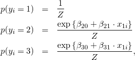
The probabilities of choosing a certain category $c$ are:

(4) $\begin{eqnarray*} p(y_i=1)&=&\frac{1}{Z}\\ p(y_i=2)&=&\frac{\mbox{exp}\left\{\beta_{20}+\beta_{21} \cdot x_{1i} \right\}}{Z}\\ p(y_i=3)&=&\frac{\mbox{exp}\left\{\beta_{30}+\beta_{31} \cdot x_{1i}\right\}}{Z}, \end{eqnarray*}$

with partiton function

$Z=1+\mbox{exp}\left\{\beta_{20}+\beta_{21} \cdot x_{1i}\right\}+\mbox{exp}\left\{\beta_{30}+\beta_{31} \cdot x_{1i}\right\}.$

Please note that $Z$ runs over all three possible states of the system.

If we write down the log-probability-ratio (or log-risk-ratio) of choosing category 2 over category 1 we get:

(5) $\begin{eqnarray*} \mbox{log}\left\{ \frac{p(y_i=2)}{p(y_i=1)}\right\}=\beta_{20}+\beta_{21} \cdot x_{1i} . \end{eqnarray*}$

From this equation the meanings of the parameters become clear. $\beta_{20}$ is nothing but the log-probability-ratio of choosing category 2 over category 1, if $x_{1i}$ is zero. $\beta_{21}$ is the expected change in terms of log-probabilty-ratios per unit increase of $x_{1i}$ .

The log-probability-ratio of choosing category 3 over category 1 is:

(6) $\begin{equation*} \mbox{log}\left\{ \frac{p(y_i=3)}{p(y_i=1)}\right\}= \beta_{30}+\beta_{31} \cdot x_{1i}. \end{equation*}$

Here we are predicting log-probability-ratios of choosing category 3 over category 1 based on the predictor $x_{1i}$ . $\beta_{30}$ is the log-probability-ratio of choosing category 3 over category 1, if $x_{1i}$ is zero and $\beta_{31}$ is the expected change in terms of log-probability-ratios per unit increase of $x_{1i}$ . Quite easy and very similar to multiple regression. The only thing one has to keep in mind is that we are predicting $C-1$ log-probability-ratios instead of changes in one continuous variable.

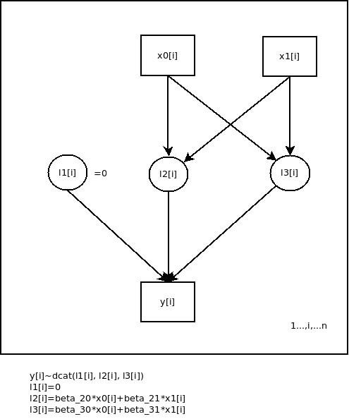
We are now in the position of having a graphical look at this simple model.

Fig. 1: Graphical representation of the simple multinomial logit regression model in the example

The variable y[i] is categorically distributed with parameters l1[i], l2[i] and l3[i]. l1[i] is set to zero for indentification purposes and l2[i] and l3[i] are linearily decomposed, e.g. due to the underlying design, if we are working experimentally. x0[i] is a dummy variable for the constants ( $\beta_{20}$ and $\beta_{30}$ ) of the regression equations and x1[i] is the predictor. The arrows symbolize dependencies between the nodes of the network.

To show how the model’s parameters of are estimated via MCMC in a Bayesian fashion, let’s introduce a little example. Let’s assume we have sampled $n=41$ individuals that are falling into two groups ( $x_i \in \left\{0,1 \right\}$ ). Each individual had the choice between 3 alternatives ( $y_i \in \left\{1,2,3 \right\}$ ). We are interested in the question: Do the groups differ with respect to the chosen alternatives? Or: Does the chosen category depend on group membership? If we crosstabulate the data in R we find:

> table(y,x)
   x
y    0  1
  1  5  3
  2 13  4
  3  2 14

By visual inspection we see that group 0 seems to have preference for alternative 2 and group 1 seems to have a preference for alternative 3. To model these data and to estimate the parameters via MCMC we have to translate the model into OpenBUGS code. This is straight forward from the graphical representation or the equations:

#uo_multinom_reg.txt
model
{
  # Likelihood
  for(i in 1:n)
  {
 
    lambda[1,i]<-0
    lambda[2,i]<-beta_20+beta_21*x[i]
    lambda[3,i]<-beta_30+beta_31*x[i]
 
    # Partition function
    Z[i]<-exp(lambda[1,i])+exp(lambda[2,i])+exp(lambda[3,i])
 
    for(c in 1:3)
    {
      p[i,c]<-exp(lambda[c,i])/Z[i]
    }
    y[i]~dcat(p[i,1:3])
  }
 
  # Priors
  beta_20~dnorm(0,1.0E-6)
  beta_21~dnorm(0,1.0E-6)
  beta_30~dnorm(0,1.0E-6)
  beta_31~dnorm(0,1.0E-6)
}

The choice of normal priors for the parameters is motivated by the theoretical result that maximum likelihood etimates are asymptotically normally distributed. In addition, the precision of the priors is set to a very low value. So these distributions encode the prior information that we really do not know anything about the distributions of the parameters in the population yet and want to let the data speak for themselves as much as possible.

The R package R2OpenBUGS is used to control the OpenBUGS script:

# uo_multinom_reg.R
library(R2OpenBUGS)
data<-read.table("uo_multinom_reg.csv", sep=",", head=TRUE)
 
# data preparation
y<-data$wahl
x<-data$geschl
n<-length(y)
 
data<-list("y","x", "n")
 
parameters<-c("beta_20", "beta_30", "beta_21", "beta_31")
 
# Initial values for the markov chains
inits <- function(){
list(beta_20 = rnorm(1), beta_21=rnorm(1), beta_30=rnorm(1), beta_31=rnorm(1))
}
 
# Handing over to OpenBUGS
output<-bugs(data, inits=inits, parameters, model.file="uo_multinom_reg.txt",
    n.chains=2, n.iter=8000, n.burnin=1000)
 
# Printing the results
print(output, digits=2)

The output of OpenBUGS is

Inference for Bugs model at "uo_multinom_reg.txt", 
Current: 2 chains, each with 11000 iterations (first 1000 discarded)
Cumulative: n.sims = 20000 iterations saved
          mean   sd  2.5%   25%   50%   75% 97.5% Rhat n.eff
beta_20   1.01 0.55 -0.02  0.64  0.98  1.36  2.13    1  2200
beta_30  -1.09 0.94 -3.22 -1.67 -1.01 -0.44  0.49    1  2600
beta_21  -0.68 1.01 -2.66 -1.35 -0.69 -0.01  1.31    1  1400
beta_31   2.78 1.16  0.76  1.98  2.68  3.48  5.35    1  2100
deviance 74.84 3.01 71.11 72.61 74.17 76.25 82.69    1 20000

For each parameter, n.eff is a crude measure of effective sample size,
and Rhat is the potential scale reduction factor (at convergence, Rhat=1).

DIC info (using the rule, pD = Dbar-Dhat)
pD = 4.1 and DIC = 79.0
DIC is an estimate of expected predictive error (lower deviance is better).

The statistics $\hat{R}$ indicate that the markov process seems to have reached a stationary distribution.

The parameter beta_20 indicates a preference of category 2 over category 1 for group 0. But this difference is statistically not significant, probably due to small sample size. beta_30 indicates a preference of category 1 over category 3 for group 0, but from the percentiles of the posterior distributions we can see that this difference is also not significant statistically.

beta_21 is the contrast of group 1 to beta_20. As we can see, group 1 seems to have a slightly lower preference for category 2 over category 1 than group 0 in terms of log-probability-ratios, but this contrast is also not significant statistically.

beta_31 is statistically significant. Group 1 has a much stronger preference for category 3 over category 1 than group 0 in terms of log-probabilty-ratios.

Please note that this setup can be extended to include a larger set of continuous and categorical predictors. Also a multilevel extension of the model seems to be straight forward by “simply” including random effects into the linear regression equations.

The main objective of this post was to show in a simple way, how categorical data analysis techniques translate into a graphical representation that in terms can be used to estimate model parameters with MCMC-methods.

Grab the code here.

Georg Hosoya

personal blog

Multinomial Logit Regression as PGM

Leave a Reply Cancel reply