The Partial Credit Model as PGM

The last post’s topic about multinomial logistic regression leads very nicely to a wide range of psychometric models for categorial responses, such as the Partial Credit Model (PCM) by Masters (1982). The PCM is a psychometric model that estimates the probability of a person’s response to an item based on characteristics of the item and the person’s latent ability. One particular nice feature of this model is the fact that Andrich’s rating scale model (RSM) and the dichotomous Rasch model (RM) are – as e.g. Mair and Hatzinger (2007) demonstrated – special cases of the PCM. It is fair to say that Samejima seems to have worked on a similar structure back in the sixties.

The focus of this post is on specifying the PCM as a graphical model, estimating the parameters via MCMC and crosschecking the results against the eRm package by Mair and Hatzinger (2007).

Let’s have a look at the formal structure of the PCM first. Starting point is the base distribution of multinomial logistic regression, sometimes called the “softmax activation function” in the machine learning literature:

(1) $\begin{equation*} p(y_i=c)=\frac{\mbox{exp}\left\{ \lambda_{ci}\right\}}{\sum_{c=1}^C\mbox{exp}\left\{ \lambda_{ci}\right\}}. \end{equation*}$

The next step is to linearily decompose the parameters $\lambda_{ci}$ with respect to the PCM. For simplicity I will consider the case of four categories per item only. Generalization to $C$ categories is simple and straight forward.

(2) $\begin{eqnarray*} \lambda_{1i}&=&0 \\ \lambda_{2i}&=&\eta_v \cdot 1 - \tau_{j,1}\\ \lambda_{3i}&=&\eta_v \cdot 2 - \tau_{j,1} - \tau_{j,2}\\ \lambda_{4i}&=&\eta_v \cdot 3 - \tau_{j,1} - \tau_{j,2} - \tau_{i,3} \end{eqnarray*}$

So, $\eta_v$ is the ability of person $v$ on the latent trait scale, and $\tau_{j,c-1}$ is the so called threshold parameter of item $j$ for the categories $c-1$ and $c$ . For example, a threshold parameter $\tau_{1,1}=-1,8$ means that for item 1, given a latent ability of $\eta_v=-1.8$ , the probability of choosing the category scored with 0 is equal to the probability of choosing the category scored with 1. This can be readily verified by for example plotting the item response functions for a set of threshold parameters. To estimate the PCM as a PGM, it is useful to introduce a multilevel perspective with respect to the persons’ abilities:

$\eta_v \sim N(0, \sigma_{\eta}^2).$

We assume that the latent abilities are normally distributed with a mean of zero and a variance of $\sigma_{\eta}^2$ , which can be estimated from data. This is actually quite nice, because approaches exist to estimate the separability or reliability based on the variance of the latent trait distribution. Please note that the parametrization of the PCM above is a bit different from the original specification by Masters (1982).

The Bugs-Code for the model is straight forward:

# PCM.txt
model{
 
  for (i in 1:n)
  {
 
        lambda[1,i]<-0
        lambda[2,i]<-1*eta[id[i]]-tau[item[i],1]
        lambda[3,i]<-2*eta[id[i]]-tau[item[i],1]-tau[item[i],2]
        lambda[4,i]<-3*eta[id[i]]-tau[item[i],1]-tau[item[i],2]-tau[item[i],3]
 
        Z[i]<-exp(lambda[1,i])+exp(lambda[2,i])+exp(lambda[3,i])+exp(lambda[4,i])
 
        for(c in 1:4)
        {
        p[i,c]<-exp(lambda[c,i])/Z[i]
        }
        y[i]~dcat(p[i,1:4])
    }
 
 
 
# Priors
  for(j in 1:k)
  {
      tau[j,1]~dnorm(0,1.0E-6)
      tau[j,2]~dnorm(0,1.0E-6)
      tau[j,3]~dnorm(0,1.0E-6)  
  }
 
  for(i in 1:N)
  {
    eta[i]~dnorm(0,tau.eta)
  }
 
    tau.eta<-pow(sigma.eta,-2)
    sigma.eta~dunif(0,2)
}

Please note that the data have to be submitted in long format.

Now, let’s do something interesting with this. The following R-script uses the rsmdat example dataset in the eRm-package, transforms it into long format and submits it to JAGS. JAGS generates the posterior distributions the Bayesian way and returns the output to R. Subsequently, the threshold- and ability-parameters are estimated with the pcm()-function in the eRm-package and the results are compared graphically.

# PCM.R
library(R2jags)
library(eRm)
 
# Load rsmdat
data<-rsmdat
# Number of thresholds per item
t<-max(data)
# Number of persons
N<-dim(data)[1]
# Number of items
k<-dim(data)[2]
# Transform data into long format
index=1
id<-c(0)
item<-c(0)
y<-c(0)
 
for(i in 1:N)
{
    for(j in 1:k)
    {
      y[index]=data[i,j]+1
      id[index]<-i
      item[index]<-j
      index<-index+1
    }
}
n<-length(y)
 
# Prepare arguments for jags()
data<-list("y","n","N","id", "item", "k")
parameters<-c("tau","eta", "sigma.eta")
inits <- function(){
list(tau = array(rnorm(t*k),c(k,t)), eta=rnorm(N), sigma.eta=runif(1)*2)
}
 
# Fit model
output<-jags(data, inits=inits, parameters, model.file="PCM.txt",
    n.chains=2, n.iter=4000, n.burnin=2000)
 
attach.jags(output)
 
# Checking against eRm ########
# Fit model with eRm
out<-PCM(rsmdat)
# Collect posterior means of threshold parameters 
# from jags output  
t1<-apply(tau[,1,],2,mean)
t2<-apply(tau[,2,],2,mean)
t3<-apply(tau[,3,],2,mean)
t4<-apply(tau[,4,],2,mean)
t5<-apply(tau[,5,],2,mean)
t6<-apply(tau[,6,],2,mean)
thresholds_pgm<-c(t1,t2,t3,t4,t5,t6)
# Collect threshold parameters from eRm
thresholds_eRm<-thresholds(out)$threshpar
# Plot PGM thresholds against eRm thresholds
plot(thresholds_eRm, ylim=c(-2,2.5), col=c("red"), ylab="tau")
points(thresholds_pgm, ylim=c(-2,2.5), col=c("green"))
 
# Collect posterior means of
# ability parameters from jags
eta_pgm<-apply(eta,2,mean)
# Collect ability parameters
# from eRm
eta_eRm<-person.parameter(out)$theta.table[,1]
plot(apply(rsmdat,1,mean),eta_eRm, xlim=c(0,3), col=c("red"), xlab="mean score",ylab="eta")
points(apply(rsmdat,1,mean),eta_pgm, xlim=c(0,3), col=c("green"))

I will spare you the outputs of JAGS and eRm but encourage you to download the scripts and to have a look yourself. Lets jump directly to the plots.

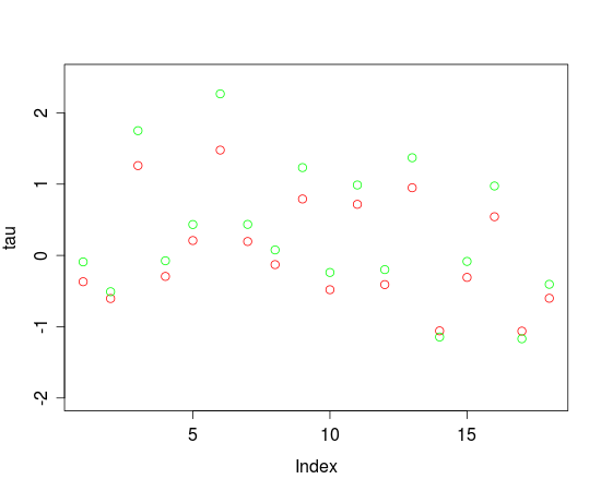
Fig. 1.: Threshold parameters estimated by eRm (red) and JAGS (green)

Visual inspection shows that eRm and JAGS essentially agree with regard to the locations of the threshold parameters. But there seems to be a difference between JAGS and eRm that is more pronounced for higher threshold parameters. The reason for this is probably the fact that JAGS samples from the posterior distributions of the parameters while eRm is using the CML-method for threshold estimation.

Let’s have a look at the ability estimates.

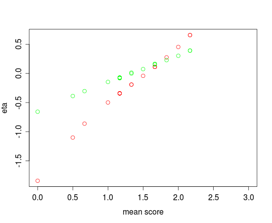
Fig. 2.: Ability estimates obtained by eRm (red) and JAGS (green) vs. mean score

In Figure 2, the differences between eRm and JAGS seem to be more pronounced. While the relationsship between the mean scores and the ability estimates seems to be more or less linear for the estimates produced by JAGS, this is not the case for eRm. The reason for this is probably the fact that the ability estimates generated by eRm were produced by using the ML-method with CML-estimates for the thresholds plugged in. Warm’s weighted ML method of person parameter estimation will most likely be included into future versions of eRm.

Which estimation method is better, Bayesian estimation with JAGS or CML combined with ML as implemented in eRm? It is hard to say from this comparison, a more systematic and thorough simulation study would be due that can be easily constructed from the code above. But note that MCMC-methods can be slow, especially for larger datasets.

The point of this post was mainly to demonstrate, how psychometric models could be fit to data with MCMC and to cross-check the results against eRm.

The scripts can be obtained here.

Georg Hosoya

personal blog

The Partial Credit Model as PGM

Leave a Reply Cancel reply